Spectral Difference Method
The SD method is an efficient high-order method for solving differential equations. We take the two-dimensional Navier-Stokes equations as an example to explain how it works. The equations can be written in the following conservative form: $$ \frac{\partial \mathbf{Q}} {\partial t} + \frac{\partial \mathbf{F}} {\partial x} + \frac{\partial \mathbf{G}} {\partial y} = 0, $$ where $\mathbf{Q}=[\rho,~ \rho u, ~\rho v,~\rho E]^\mathsf{T}$ is the vector of conservative variables, $\mathbf{F}=\mathbf{F}_{inv}+\mathbf{F}_{vis}$ and $\mathbf{G}=\mathbf{G}_{inv}+\mathbf{G}_{vis}$ are the flux vectors. The subscripts '$inv$' and '$vis$' stand for 'inviscid' and 'viscous', respectively. These flux vectors have the following expressions, $$ \mathbf{F}_{inv} = \left[ \begin{array}{c} \rho u \\[0.3em] \rho u^2 + p \\[0.3em] \rho uv \\[0.3em] (\rho E+p)u \end {array} \right], ~ \mathbf{F}_{vis} =-\left[ \begin{array}{c} 0 \\[0.3em] \tau_{xx} \\[0.3em] \tau_{yx} \\[0.3em] u\tau_{xx}+v\tau_{yx}-q_x \end{array} \right], ~ \mathbf{G}_{inv} = \left[ \begin{array}{c} \rho v \\[0.3em] \rho uv \\[0.3em] \rho v^2 + p \\[0.3em] (\rho E+p)v \end {array} \right], ~ \mathbf{G}_{vis} =-\left[ \begin{array}{c} 0 \\[0.3em] \tau_{xy} \\[0.3em] \tau_{yy} \\[0.3em] u\tau_{xy}+v\tau_{yy}-q_y \end{array} \right]. $$
In SD method on quadrilateral meshes, each mesh element is mapped from the physical space $(x,y)$ to a standard unit square element in the computational space $(\xi,\eta)$ using, for example, iso-parametric mapping.
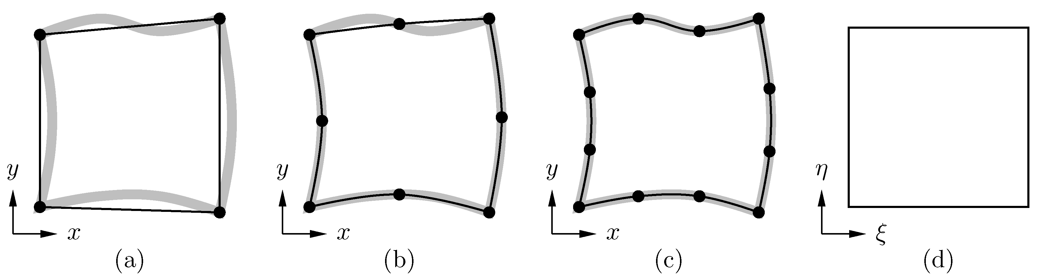
The mapping also transforms the Navier-Stokes equations into the following conservative form in the computational space:
$$
\frac{\partial \widetilde{\mathbf{Q}}} {\partial t} + \frac{\partial \widetilde{\mathbf{F}}} {\partial \xi} + \frac{\partial \widetilde{\mathbf{G}}} {\partial \eta} = 0,
$$
where $\widetilde{\mathbf{Q}}$, $\widetilde{\mathbf{F}}$ and $\widetilde{\mathbf{G}}$ are the computational solution and flux vectors that are related to the physical ones as
$$
\widetilde{\mathbf{Q}} = |\mathcal{J}|\mathbf{Q}, ~~
\left( \begin{array}{c} \widetilde{\mathbf{F}} \\[0.3em] \widetilde{\mathbf{G}} \end{array} \right) = |\mathcal{J}|\mathcal{J}^{-1}
\left( \begin{array}{c} \mathbf{F} \\[0.3em] \mathbf{G} \end{array} \right),
$$
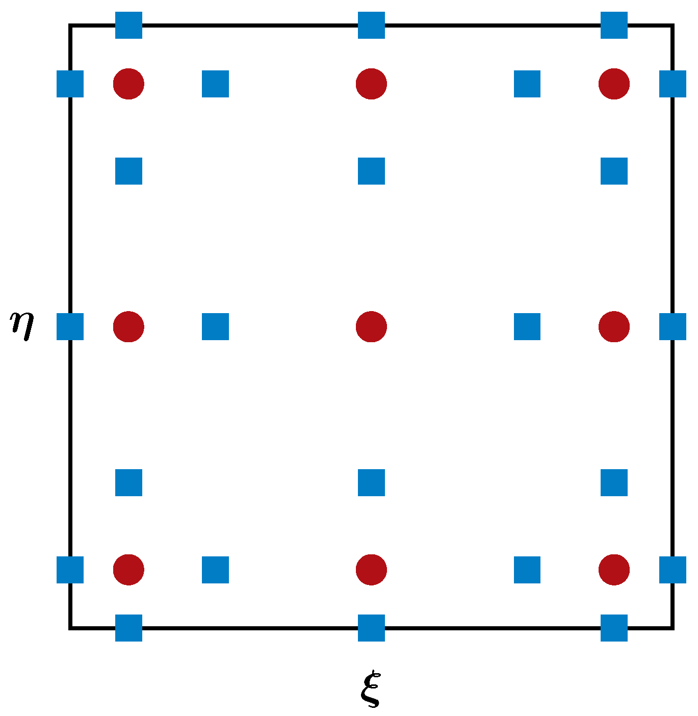
where $\mathcal{J}=\partial (x,y)/\partial (\xi,\eta)$ is the Jacobian matrix for the mapping, $|\mathcal{J}|$ is its determinant, and $\mathcal{J}^{-1}$ is its inverse. Solution points (SPs) $X_s$ and flux points (FPs) $X_{s+1/2}$ are then defined within each standard element to facilitate the construction of solution and flux polynomials. The figure below sketches the distribution of the SPs and FPs for a third-order scheme, where the red circular dots denote the SPs and the blue square dots denote the FPs.
 With these points defined, the following Lagrange interpolation bases are readily available at each SP and FP in a standard element,
$$
h_i(X) = \prod_{s=1,s\neq i}^{N}\left(\frac{X-X_s}{X_i-X_s}\right), ~~
l_{i+1/2}(X) = \prod_{s=0,s\neq i}^{N}\left(\frac{X-X_{s+1/2}}{X_{i+1/2}-X_{s+1/2}}\right).
$$
They are employed to construct the solution and flux polynomials through tensor products as below,
$$
\begin{aligned}
\widetilde{\mathbf{Q}}(\xi,\eta) &= \sum_{j=1}^{N} \sum_{i=1}^{N} \widetilde{\mathbf{Q}}_{i,j} h_i(\xi) h_j(\eta), \\[0.5em]
\widetilde{\mathbf{F}}(\xi,\eta) &= \sum_{j=1}^{N} \sum_{i=0}^{N} \widetilde{\mathbf{F}}_{i+1/2,j} l_{i+1/2}(\xi) h_j(\eta), \\[0.5em]
\widetilde{\mathbf{G}}(\xi,\eta) &= \sum_{j=0}^{N} \sum_{i=1}^{N} \widetilde{\mathbf{G}}_{i,j+1/2} h_i(\xi) l_{j+1/2}(\eta).
\end{aligned}
$$
The above polynomials are only element-wise continuous, but discontinuous across element boundaries. Therefore, common solutions and common fluxes need to be defined on element boundaries. These common values are computed, for instance, by averaging and by using a Riemann solver, etc. Once the common values are obtained, one can compute the residuals by directly differentiating the then continuous polynomials, and then update the solutions using a time-marching scheme.
With these points defined, the following Lagrange interpolation bases are readily available at each SP and FP in a standard element,
$$
h_i(X) = \prod_{s=1,s\neq i}^{N}\left(\frac{X-X_s}{X_i-X_s}\right), ~~
l_{i+1/2}(X) = \prod_{s=0,s\neq i}^{N}\left(\frac{X-X_{s+1/2}}{X_{i+1/2}-X_{s+1/2}}\right).
$$
They are employed to construct the solution and flux polynomials through tensor products as below,
$$
\begin{aligned}
\widetilde{\mathbf{Q}}(\xi,\eta) &= \sum_{j=1}^{N} \sum_{i=1}^{N} \widetilde{\mathbf{Q}}_{i,j} h_i(\xi) h_j(\eta), \\[0.5em]
\widetilde{\mathbf{F}}(\xi,\eta) &= \sum_{j=1}^{N} \sum_{i=0}^{N} \widetilde{\mathbf{F}}_{i+1/2,j} l_{i+1/2}(\xi) h_j(\eta), \\[0.5em]
\widetilde{\mathbf{G}}(\xi,\eta) &= \sum_{j=0}^{N} \sum_{i=1}^{N} \widetilde{\mathbf{G}}_{i,j+1/2} h_i(\xi) l_{j+1/2}(\eta).
\end{aligned}
$$
The above polynomials are only element-wise continuous, but discontinuous across element boundaries. Therefore, common solutions and common fluxes need to be defined on element boundaries. These common values are computed, for instance, by averaging and by using a Riemann solver, etc. Once the common values are obtained, one can compute the residuals by directly differentiating the then continuous polynomials, and then update the solutions using a time-marching scheme.